End User Friendly Conditional Formatting

This is one of the major new features of LL21. Conditional Formatting is needed whenever you want to change properties depending on data, e.g. something like "red font if value is negative" or "highlight the background if value is greater than threshold". This allows to read a report at a glance and quickly get an overview of what areas of your data require a second look.

Of course, this can also be done in LL20, but it requires some knowledge of properties and formulas. You need to find the font color property, figure out how to use a formula for it and use a Cond() function that does the handling. If you want to add more conditions (e.g. bold font for one threshold and a highlight color for another), you quickly end up with a nested Cond() statement that can get quite complicated. The average end user will probably not be able to handle this gracefully.

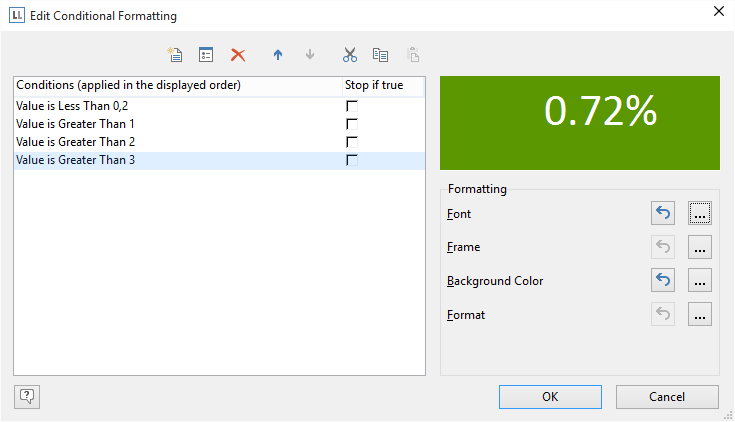
Enter the brand new Conditional Formatting feature. This is a great way to combine easily accessible formatting rules in one place. You can enter cascades of conditions and you can even tell LL21 if a rule should stop further processing once it matches or if other rules should be processed additionally. For each value type there are loads of handy presets that make defining conditional formattings a piece of cake.

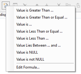
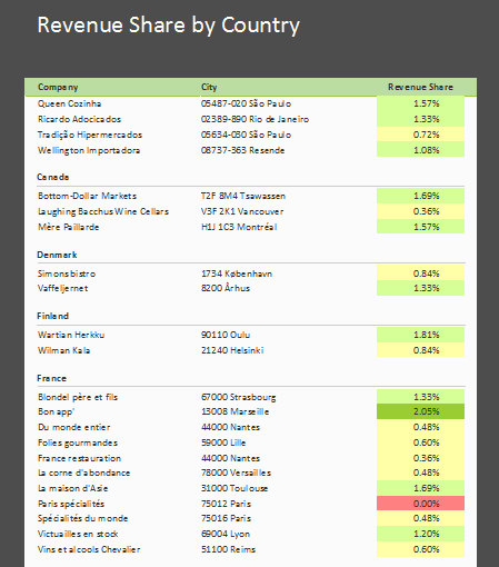
Let’s do a quick walkthrough – imagine a customer list where you want to color-code the customers depending on their revenue share. You want different colors for shares below 0.2% (reddish) and those above 1%, 2%, and 3% (different greens). If you don’t have the revenue share in your database, it could e.g. be calculated using the native aggregate functions I’ve blogged about before.

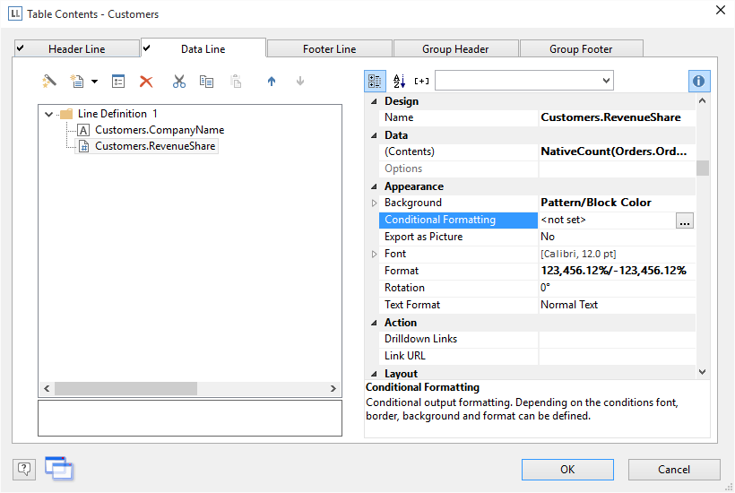
The table column now has a new property “Conditional Formatting”:
 

New feature of version 21
 

Clicking on the “…” for the “Conditional Formatting” property of the revenue share column gives you the following dialog:
 

New feature of version 21

Now insert a new condition – a dropdown appears that presents you with a number of useful templates:
 

New feature of version 21
 

Choose the “Value is Greater Than…” template and enter the required number in the following dialog:
 

New feature of version 21
 

Now click on the “…” for the background property and choose the color as required:
 

New feature of version 21
 

That’s it – adding the other conditions is quickly done following the same procedure. For this example, a darker green should be chosen for each percentage. For the >3% formatting, you could also change the font’s color to white, as the contrast will look much nicer then. To do so, simply click the “…” for the conditional formatting’s font style and select the required color:
 

New feature of version 21
 

Note the consistent usage of the new color picker UI throughout all dialogs – LL21 has really been streamlined for end user usability. This will make your application shine in the end user’s eyes. The Conditional Formatting dialog finally looks like this:
 

New feature of version 21
 

And the final color coded report allows to see at a glance which customers have the largest revenue shares:
 

New feature of version 21
 

The same works for date and text columns, including suitable templates like date ranges or “Starts with” conditions. Conditional Formattings can also be applied to text object paragraphs and crosstab cells. They are a very user friendly, intuitive way to achieve what needed complex, nested formulas before or even was downright impossible.
 

Related Posts

Leave a Comment